meta data for this page
Description of functions
2.1 Creation of graphic data
To create the required graphic data a Twain interface is provided. By means of this interface all optical devices such as scanner, digital cameras, video cameras or microscopes can be controlled by the program.
2.2 Selection of devices
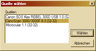
To select the needed Twain device you have to use the menu item File > Select Source. A window appears listing all existing devices.
Figure 1. Device selection window
2.3 Scan
Use the menu item File > Scan in order to open the desired device program for the creation and export of image files.
Figure 2. Scan mask
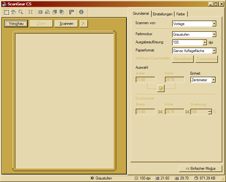
In figure 2 a control program of a Canon colour picture scanner is shown.
Detailed operating instructions have to be extracted from the program documentation of the producer.
In general you have to consider which colour mode or resolution of the target file is selected. The colour mode selection depends on how individual image objects differ from each other. If
a greyscale analysis allows a clear differentiation so the mode Greyscale can be reasonable. Otherwise the mode Colour has to be selected.
Concerning the image resolution you have to take into account that a higher resolution leads to a more precise analysis on the one hand. On the other hand it requires a longer processing time and more memory capacity.
Devices used for enlarging images (e.g. microscope) require the input of a magnification factor. A corresponding window appears automatically or can be opened by the menu item Options > Magnification factor (see chapter 6.7).
Figure 3. Input mask – magnification factor

Figure 4. Control mask - Mikokular (microscope)
If the magnification factor is unknown, such as at photographs made by a digital camera, it is necessary to take a test photo with a scale (e.g. ruler). The magnification factor then can be determined on the basis of the difference between the scale and the length measuring of the scale done by the program after scanning (see chapter 4.3).
2.4 Twain input mask
To use the Twain input mask of the selected Twain device you have to activate the option File > Show twain input mask. Otherwise it is tried to import the image on the basis of standard settings :
Scanner (default):
• resolution 100 dpi
• colour depth 24 Bit
• width 210 mm
• length 297 mm
Mikrokular (microscope)
• resolution 320 x 240 dpi
• colour depth 24 Bit
2.5 Filemanagement
2.5.1 Open files
By default the image file format MYP is offered. MYP is a program internal format, including a packed image without loss and additional needful information such as the magnification factor and more. Image files of the formats BMP and JPEG can be loaded too. In this case parameters concerning resolution, colour depth (menu item Options > dpi and resolution) or magnification factor have to be defined manually (see chapter 6.6 and 6.7).
2.5.2 Close files
By default image files are stored in the format MYP (see chapter 2.5.1).
It is also possible to store it in a BMP format, but then all additional parameters (magnification factor …) get lost.
Please note: The image of the work space is stored in WYSIWYG mode. If the image should have been changed, these changes are stored too, e.g. raster display or display mode black/yellow (see chapter 6.3 and 3.2).
2.6 Create image objects
This function provides the area computation of objects whose contours are captured by a graphic input device.
2.6.1 Create images
To create the image please select the menu item File > Create.
Figure 4.: Creation of an image

The creation of a drawing area (A2 – A5) requires a calibrating of the input device (see Calibrate input device ).
2.6.2 Calibrate input devices
With this function the resolution capability of the mouse is determined (DPI) .
Figure 5.: Calibrate the input device
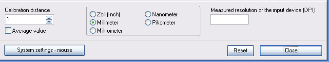
1. Select calibration distance and unit
2. Press the left mouse button and go along the section of measurements
Press the button System parameters mouse in order to configure the mouse, if the resolution of the mouse should be too large. A DPI value bigger then 500 leads to a slowdown of the program execution, because the image size has to be matched with these settings.
Select the button Finish Calibration for applying the determined settings.
2.6.3 Draw objects
It is possible to draw objects either on an empty work space (format DIN A2 – A5) or on a loaded template.
Objects can be generated by two different methods :
1) Freehand
2) Connected lines
1) Freehand
Set the mouse on the object (arrow or the like) first, press the left mouse button then and go around the object with the mouse button keeping pressed.
After releasing the button the starting point will be connected automatically with the end point and the object is filled.
Please note : The starting point is located in the upper left region of the drawing area. The visible changes automatically when drawing (within the format definition A4, A5…). If the defined working space is left while drawing a system tone raises.
Press the button Apply to make the created image available in the main program (only available in a full version) for an automatic computation of the object area.
2) Connected lines
Set the mouse on the object and press the left mouse button. The starting point is marked on the drawing area as a small black point. Move the mouse to the next object point and press the left button. The points are connected automatically. Additional points have to be marked in the same way.
Press the right mouse button at last to connect the starting and end point. The object is filled automatically.
Please note : Keep the left button pressed to activate the auto scroll function. In this case press the right button to mark single points. Both buttons have to be released to finish the process. Press the right button once again and the object will be shown as described above. If the defined work space is left a system tone raises.
Press the button Apply to transfer the created image to the main program (only available in a full version) for an automatic computation of the object area.
The NUM buttons 4,8,6 and 2 can also be used for scrolling.
2.7 Video interface
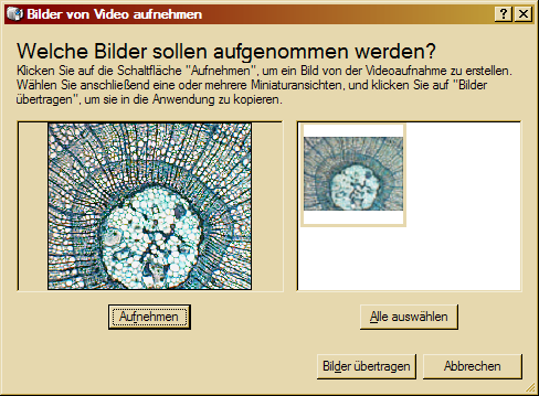
As shown in figure 8 it is possible to import images directly
by diverse video equipment such as frame grabber, video grabber etc.
Figure 6. Video
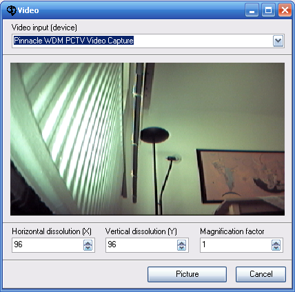
Select the desired video input and please enter the camera resolution
and magnification factor into the provided fields (seel also chapter
7.2 Calibration). Press then the button \’Picture\’ to import
the image as a snapshot in your programme.
2.8 Stack processing
In stack processing mode multiple images (e.g. image sequences) can be opened concurrently in a stack. The target is to generate a new image resulting from multiple source images.
Figure 7. Opening in batch mode
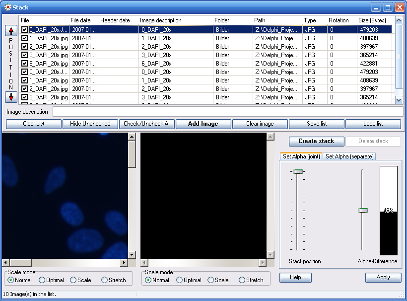
2.8.1 Data file list
An unlimited number of images can be listed to generate the desired image stack. The list entries can be sorted either automatically (click on column header) or manually (use right mouse button or button on the left side of the table or function keys F5 to F8). It is furthermore possible to rotate an image within the defined stack. To display an image on the monitor on the left side simply click on the corresponding list entry. All created lists can be stored for later processing.
2.8.2 Create a stack
With a click on the button “Create stack” all images of the list will be merged into a stack in the given order. The result is to be seen on the monitor on the right.
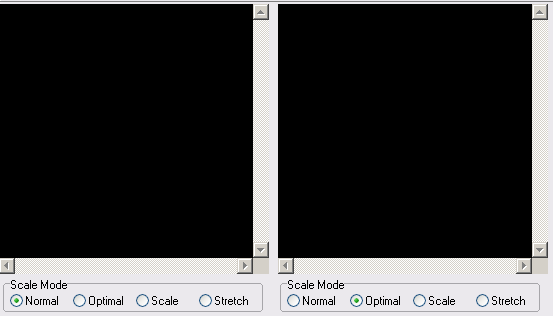
2.8.3 Monitor windows
The monitor windows are intended to control images respectively to select images from the list. Several options for image scaling are offered. The mode “Scale” allows to zoom in and out by the function keys F9 or F10.
Figure 8: Monitor windows
2.8.4 Changing alpha values in the stack
It is possible to change the visibility (alpha values) of single stack images in order to create individually a new image.
2.8.4.1 To change alpha values harmonically
Figure 9: To change alpha values harmonically

With the left slide control it is possible to define the master image of the stack. For example, there are 10 images in the stack and the controller is at five, that means the 5th image is fully visible. All other images, lying before or behind, are damped visible corresponding to the slider on the right. Concerning our example we have the following alpha-values:
Image 1 : 0; Image 2 : 21; Image 3 : 99; Image 4 : 177; Image 5 : 255
Image 6 : 177; Image 7 : 99; Image 8 : 21; Image 9 : 0; Image 10 : 0
That means, the images 1, 9 and 10 will have no influence on the resulting image.
By moving the left slider you can go through the stack. The image blending is, corresponding to the setting of the right slider, more or less fluently (on 100 % the master image is equal to the output image).
2.8.4.2 To change alpha values individually
Figure 10: To change alpha values individually
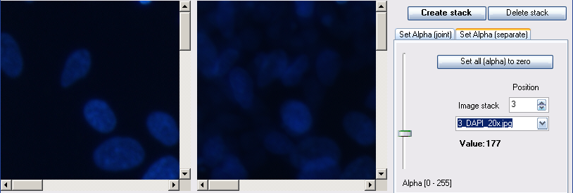
With this setting you are able to set alpha values for every single image of the stack individually. The result (a blended image) is displayed in the right monitor window. An alpha value of 255 means a high visibility, 0 means invisibility.
2.8.5 To apply an image for the purpose of analysis
After the completion of the image the result can be transferred to the main program. Press the button “Apply” to do so. You then will be asked to enter the image resolution, the file type and the used image magnification manually. These values are the basis for the following area or length calculation .
2.8.6 To change the location of images from stack
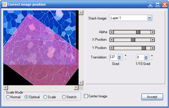
It is possible to manipulate the location of all stack images to one another. For this purpose the serveral layers can be selected by a combobox. The images can be relocated in X/Y direction and also be rotated. The smallest rotation angle is 1/10 degree.
Figure. To change location